CIS 558 / Linguistics 525
Computer Analysis and Modeling of Biological Signals and Systems
Homework 1
Due: 2/5/1999
This set of exercises corresponds roughly to the first two items in the syllabus.
Thus it is due at the end of the fourth week of the course. However, it is strongly
suggested that you begin earlier, doing one section each week.. If you run into
any troubles, either technical or conceptual, please contact me.
The Matlab instructions are for Unix, and specifically for the (clients of)
unagi.cis. If you are doing the homework in one of the PC labs, or elsewhere
on campus, contact me in advance in order to ensure that the needed data
files are available to you, and that any necessary changes in instructions are
specified.
In order to access the referenced Matlab objects, make a directory ~/matlab
(in your home directory), create a file called startup.m in your matlab
directory, and add to it a line such as
path(path,'/mnt/unagi/speech/matlab')
Except for section III, questions 1 and 2, your answers should be in the form
of a file that can be executed directly by Matlab. Please check that your file
can actually be executed before submitting it. Email your solutions to myl@unagi.cis.
If you want to add any commentary, use the comment character % to do
so. For III/1-2, your answer can be in the form of Matlab comments; Matlab code
for this case is optional.
I. Using MATLAB
A. Basic 1D operations in MATLAB
- The file audio1.mat contains 10,399 numbers representing about 1.3
seconds of a sound waveform sampled 8,000 times a second, assigned to a variable
named S. Load it using the command load('audio1')
Now plot the vector S. Use the Matlab function plot. You
can execute help plot to get information on this function.
- Given that S is sampled at 8 KHz, with the first sample representing time
1/8000 and the 8000th sample representing time 1, create a second vector of
the samples spanning the time period from .275 to .325 seconds inclusive.
Plot it. Keep in mind that putting a semicolon after a MATLAB expression will
prevent its value from being printed.
- Create a third vector corresponding to the 10399 samples of S scaled so
that the minimum value is -1 and the maximum value is 1.
- Calculate the serial cross-correlation of 80-sample pieces of S, starting
at sample 2200, for lags between 1 and 150 samples inclusive. In other words,
calculate a vector A such that

You can do this using the MATLABfor loop and the functions sum
and sqrt. More efficiently, try to use your knowledge of linear algebra
(inner products, vector lengths)!
As the nomenclature implies, you are calculating the correlation of a
piece of S with another piece of S at a variety of offsets. Calculations
of this kind are used in periodicity detection. Keep in mind that Matlab's
vector indices start with 1 rather than 0.
- What is the maximum value of A? For what index value does it occur? Use
help max to see how to find this out.
- Plot A three times, first with the X axis in samples; second with the X
axis in seconds (i.e. samples/8000); and third with the X axis in Hertz (the
inverse of the measure in seconds). In the last case, limit the range of values
shown to 500 Hz. and below.
- [Extra Credit] Calculate a version of A based only on the numerator of the
equation given (i.e. based only on the inner products of an 80-element stretch
of S with 150 other 80-element stretches of S. Is the maximum at a different
place?
B. Basic 2D operations in MATLAB
The following problems pertain to image-processing in Matlab. An image is
stored as a two-dimensional matrix, and displayed with the command image.
The elements of the image are typically called ``pixels''. A modified version
called imagesc will scale the pixel values so that the largest is mapped
to white and the smallest to black.
Execute the following to load an image into Matlab from the course directory:
fid = fopen('einstein.raw','r')
al = fread(fid,[256,256],'uchar')';
fclose(fid)
Now display the image using imagesc. You may also have to
execute the expression colormap(gray).
- Select a subimage of al with vertical indices in the range 70-120
and horizontal indices in the range 80-130. This operation is commonly refered
to as ``cropping''. Display the subimage. Note that even though the subimage
is smaller than the original, it is displayed as being the same size (Note:
you can use the command size to determine the actual size of the
underlying pixel array). Why is this? What happens when you resize the Matlab
figure window?
- Create an image containing every fourth pixel (in both the
horizontal and vertical directions). This operation is known as
``subsampling'' (Hint: check the help information for colon).
- Create a vector containing the 25th row of al.
Plot it.
- Compute the minimum and maximum values of al. At what locations
do these occur? Plot a histogram (essentially, a probability distribution)
for the pixel values of al using the Matlab function hist.
- Matlab allows us to operate on images point-by-point. Compute (and display)
a new image whose pixels are the square root of the pixels of al.
Look at the histogram and compare it to that of al (you may want
to execute the command figure(2) to put this in another window).
Compute and display an image containing a pixel of value 1 at locations where
al is greater than 128, and 0 elsewhere.
- Load another image from the file 'reagan.raw' in the course
directory. Compute images that are the sum and product (pointwise!)
of this image and al.
II. Color Matching
Execute the command load('colmatch.mat') in your Matlab environment.
This file contains a number of matrices and vectors related to the color matching
problems discussed in class. In particular, the variable P is
an N x 3 matrix containing wavelength spectra for three basis lights
(``primaries''), and the variable M is a 3 x N color-matching
matrix corresponding to these primaries. For these problems N=31, corresponding
to samples of the wavelength spectrum from 400nm to 700nm in increments of 10nm.
Set the variable light to a random vector of length 31. We
will consider the components of this vector to be samples of the wavelength
spectrum of a particular light.
- What combination of the three primaries in P will match the
appearance of this randomly chosen test light? Compute the wavelength spectrum
of the matching light (as a linear combination of the three primary wavelength
spectra) and compare it to that of the test light. Why is it different?
- The variable Palt contains a different set of primary lights.
Compute the corresponding matching matrix Malt (you will probably
need to make use of the Matlab function inv which computes the inverse
of a square matrix). Repeat the previous exercise with Palt
and Malt. Is the matching spectrum different than in the previous
exercise?
- The variable Phosphors contains the emission spectra of
three standard color monitor phosphors. How would you choose the amplitude
of each phosphor's emission in order to produce light on the monitor that
matches light? Compute these amplitudes and demonstrate that
the resulting mixture of phosphors does indeed produce the same tri-stimulus
coordinates in the matching experiment.
- The variable M2 contains yet another matching matrix. This
one was computed for a color-impaired individual, using the primaries in P.
Compute the SVD of M2. How can you tell this individual is
color-impaired? Assume that the individual has a standard color-blindness
problem: they are missing one or more cone types. Derive the spectral sensitivity
of the missing (or remaining) cone.
- The variable Cones contains approximate spectral sensitivities
of t he three color photoreceptors (cones) in the human eye. They are ordered
such that Cones(1,:) corresponds to the L (long-wavelength, or red)
cones, Cones(2,:) the M (green) cones, and Cones(3,:) the
S (blue) cones. Plot these using plot or try rgbplot, and
compare to the cone sensitivity vector you derived in the previous problem.
Which cone was missing from (or remaining in) your color-blind subject?
- Having just purchased a new house in Center City, you decide to
paint the baseboard trim a new color. In particular, you'd like to
have the trim match the color of your new couch (chartreuse, of
course). You make a trip to the paint store, carrying with you a
sample piece of fabric (complete with plastic slipcover). The store
carries two brands of paint: ShabbyTint, which is mixed from
three primary colors, and RichTone, which is mixed from a set of six
primary colors. Naturally, the RichTone costs four times as much, so
you decide to go with the ShabbyTint, and quickly pick a matching
color from the ShabbyTint paint chart (the store mixes it for
you, from the three ShabbyTint primaries).
Load the file paint.mat into Matlab. This will define a few variables:
- couch contains a vector of the color reflectance function
of the couch.
- shabby is a matrix whose columns are the reflectance
functions of the three ShabbyTint primaries.
- rich is a matrix whose columns are the reflectance
functions of the six RichTone primaries.
- fluo contains a vector of the color spectrum of the
fluorescent lights in the paint store, and in your living room.
- daylight contains a vector of color spectrum of the
sun.
- Determine the mixture of ShabbyTint primaries that will match
the sample you've taken to the paint store. Assume that paint-mixing is
additive (it really isn't!). Plot the wavelength spectra of the sample
and the paint (when viewed in the paint store) on the same plot (use the
Matlab hold command to do this). Demonstrate that a paint mixed
from this proportion of the three primaries will look just like the sample.
- You may now view these colors on your monitor. Create two column vectors
of height 3, called rgb1 and rgb2 containing
the monitor gun values (proportion of each phosphor) to be used to display
a color matching the couch and the shabby paint mixture under fluorescent
lighting. You should assume that the matrix Phosphors contains
emission spectra that are correct for your monitor (this may not be true).
Then call the function
showcols(rgb1,rgb2).
- You take the paint home, and paint a small sample of baseboard.
The next morning, when the sun comes up, you
find to your horror that the baseboard doesn't match the couch at all.
What happened? Show that the two colors really don't match when
viewed under daylight. Render them on the screen using
showcols to check this.
- What is the best (least-squares) combination of ShabbyTint primaries
that you could have used to match the couch both in daylight and incandescent
light?
- What if you use the RichTone paint? Assess the quality
of the best-matching mixture under both daylight and fluorescent light.
III. Linear Shift-Invariant Systems
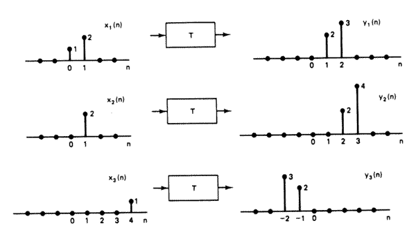
- (Oppenheim and Shafer 1989 p. 68). The system T in the figure below is
known to be time-invariant. When the inputs to the system are x1[n], x2[n]
and x3[n], the responses of the system are y1[n], y2[n], y3[n] respectively.
- Could the system T be linear? Explain.
- If the input x[n] to the system T is delta[n] (i.e. a unit impulse
at time 0), what is the system response y[n]?
- Determine all possible inputs x[n] for which the response of the system
T can be determined from the given information alone.

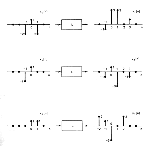
- (Oppenheim & Shafer 1989 p. 69) The system L in the figure below is
known to be linear. When the inputs to the system are x1[n], x2[n], x3[n],
the response is y1[n], y2[n], y3[n] respectively.
- Could the system L be time-invariant? Explain.
- If the input x[n] to the system is delta[n], what is the system response?

- Create a vector of length 24 containing an impulse at location 5, a step
edge at location 12, and a unit-slope ramp starting from location 18. Convolve
this signal with the ``two-point averager'': [0.5, 0.5], and the
``two-point differencer'': [0.5,-0.5]. How does the differencer respond
to the various features?
- Show that the two convolution results computed above may be added together
to reconstruct the original signal. Would this be true for an arbitrary input
signal?
- Write a Matlab function mksine to construct a vector of samples
of a sine function. The function should take arguments size, period,
amplitude, and phase. The phase should be measured from
the first sample (that is, the first sample is at the origin).
- Compute the convolution of each of two 24-sample sinusoids of period 24
and period 4 with the two filters described above. Note the amplitude of the
results. What can we conclude about this ``decomposition''?
- Load images ``al'' and ``ron''. Compute a 3-point horizontal weighted average
of al using the kernel [ 0.25 0.5 0.25 ]. Compute a similar 3-point
vertical average.
- Now convolve with both filters (sequentially). What equivalent single 2D
convolution would produce the same result (give the convolution kernel, and
show that the result is the same)?
- The result of this convolution may not look so different from the original,
but try subtracting it from the original. What equivalent single 2D convolution
would have produced this result?
- Take the result of the previous part (difference of original and average),
and compute the following binary image:

Could we have computed it via a single convolution?
- Write a function mksine2 that constructs an array of samples from
a 2D sine wave. This function should take similar arguments, but will require
both xsize and ysize, and should also take an angular argument
direction specifying the normal direction of the sine wave.
Mark Liberman
1/18/1999


