Analysis of variance
Searching Google Scholar for "Analysis of Variance" produces 850,000 hits.
There are many variations on the ANOVA theme, and most of them are fairly easy to understand in a procedural sense. It's often harder to understand why a particular set of procedures should be followed, and how to interpret the results. But it's all the more important to understand the procedures in detail, with all their their assumptions, rather than simply to plug some data into a program and copy the resulting magical formula (F(1,38)=8.7, P < 0.01, η2=0.186) into your paper.
The development of ANOVA and related techniques was historically associated with the development of experimental design, and especially with factorial experiments. 80 years ago, it was a radical step when R.A. Fisher wrote (in "The arrangement of field experiments", Journal of the Ministry of Agriculture of Great Britain 33:503-513, 1926):
No aphorism is more frequently repeated in connection with field trials, than that we must as Nature few questions, or, ideally, one question, at a time. The writer is convinced that this view is wholly mistaken. Nature, he suggests, will best respond to a logical and carefully thought out questionnaire; indeed, if we ask her a single question, she will often refuse to answer until some other topic has been discussed.
Today, Fisher's ideas about how to design a "logical and carefully thought out questionnaire", and how to interpret Nature's answers, have become conventional wisdom among scientists in many disciplines. The radicals today are those who say things like this (R. Harald Baayen, "Statistics in Psycholinguistics: A critique of some current gold standards", Mental Lexicon Working Papers I, 2004):
The most commonly used statistical technique in psycholinguistics is analysis of variance. Generally, experimental research is planned in terms of factorial contrasts. Factorial designs are widely believed to be superior to multiple regression. Learning how to construct a data set with a factorial contrast while matching for a range of continuous predictors such as frequency of occurrence is regarded as an essential skill for experimental studies. As most psycholinguistic studies present a range of items to many different subjects, experimental data sets routinely undergo the averaging procedures of the by-subject and by-item analyses, applied indiscriminately not only to continuous variables such as response latencies, but also to dichotomous variables such as the accuracy measure. Many researchers seem to believe that the accepted statistical methods currently in use, and generally enforced by the journals, are the best that modern statistics has to offer.
The purpose of this study is to question the validity of this cluster of ideas and assumptions.
I would add that in the case of language, Nature is generally ingenious in devising barriers to factorial design, by arranging for factors to be intricatedly entangled, if only by virtue of the fact that most quantities of interest follow LNRE ("large numbers of rare events") distributions. Attempts to thwart this aspect of Nature's design can fail in both obvious and also unexpected ways. [More on this later.]
For general background on sums-of-squared-deviations, check out the Wikipedia article. Then try downloading and running Atest.m and Atest1.m, modifying them and re-running them until you're sure that you understand what's happening.
Now let's look at one of Fisher's own examples of a "logical and carefully thought out questionnaire". As you'll see, the calculations are all very simple ones -- the only complexity is knowing which calculations to make. Well, and the result is a ratio (e.g. 3.967/.727 = 5.4567) which we need to compare to a threshold given to us by an oracle (e.g. finv(.95,11,24) = 2.2163), in order to decide whether a celebration is propitious.
The example is taken from R.A. Fisher, Statistical Methods for Research Workers, 1925; Chapter 7, "Intraclass correlations and the analysis of variance":
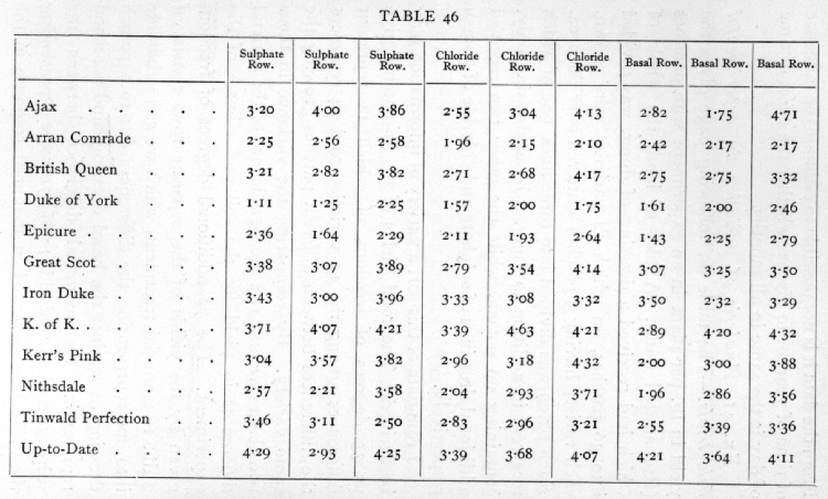
A plot of land, the whole of which had received a dressing of dung, was divided into 36 patches, on which 12 varieties [of potatoes] were grown, each variety having 3 patches scattered over the area. Each patch was divided into three lines, one of which received, in addition to dung, a basal dressing only, containing no potash, while the other two received additional dressings of sulphate and chloride of potash respectively.
Nature's answer to this agricultural questionnaire is a 12-by-9 table of potato weights ("yield in lbs. per plant"):

The idea is to determine whether these varieties have different yields, whether these treatments make a difference, and whether the treatments make a different amount of difference for different varieties of potatoes.
Keep in mind, as you read on, that Fisher frames (and evaluates) the questions entirely in terms of "statistical significance": how likely are the observed numbers to have arisen by chance in an experiment where there are no underlying effects (of variety or treatment or their interaction), but only sampling error?
This is worth knowing, but it's arguably not as important as estimating how big the effects are, and how much relevant gain or loss is associated with them. An effect may be highly "significant", in the sense that it is vanishingly unlikely to have arisen as a result of sampling error, but completely insignificant in the sense that its magnitude is tiny in the context of the phenomena of interest.
Fisher tells us:
From data of this sort a variety of information may be derived. The total yields of the 36 patches give us 35 degrees of freedom, of which 11 represent differences among the 12 varieties, and 24 represent the differences between different patches growing the same variety. By comparing the variance in these two classes we may test the significance of the varietal differences in yield for the soil and climate of the experiment.
Now Fisher is going to calculate the numbers that the Wikipedia article calls I, T, and C.
The sum of the squares of the deviations of all the 108 values from their mean is 71.699; divided, according to patches, in 36 classes of 3, the value for the 36 patches is 61.078; dividing this again according to varieties into 12 classes of 3, the value for the 12 varieties is 43.638·
Let's try to reproduce these values in Matlab. First, we enter the potato data:
FP = [3.20 4.00 3.86 2.55 3.04 4.13 2.82 1.75 4.71 ; ...
      2.25 2.56 2.58 1.96 2.15 2.10 2.42 2.17 2.17 ; ...
      3.21 2.82 3.82 2.71 2.68 4.17 2.75 2.75 3.32 ; ...
      1.11 1.25 2.25 1.57 2.00 1.75 1.61 2.00 2.46 ; ...
      2.36 1.64 2.29 2.11 1.93 2.64 1.43 2.25 2.79 ; ...
      3.38 3.07 3.89 2.79 3.54 4.14 3.07 3.25 3.50 ; ...
      3.43 3.00 3.96 3.33 3.08 3.32 3.50 2.32 3.29 ; ...
      3.71 4.07 4.21 3.39 4.63 4.21 2.89 4.20 4.32 ; ...
      3.04 3.57 3.82 2.96 3.18 4.32 2.00 3.00 3.88 ; ...
      2.57 2.21 3.58 2.04 2.93 3.71 1.96 2.86 3.56 ; ...
      3.46 3.11 2.50 2.83 2.96 3.21 2.55 3.39 3.36 ; ...
      4.29 2.93 4.25 3.39 3.68 4.07 4.21 3.64 4.11 ];
("FP" stands for "Fisher's Potatoes".)
Now the "sum of the squares of the deviations of all the 108 values from their mean":
>> x = FP-mean(FP(:)); sum(x(:)'*x(:))
ans =
   71.6989
Remember that x(:) is Matlab-ese for turning a matrix into a vector; and note that Fisher is dealing in sums of squared deviations, not variances, for which we'd have to divide by the number of elements involved.
And note that we could also get this number by subtracting the "Composite" sum of squares (the square of the overall sum, divided by the number of cases) from the "Individual" sum of squares:
II = FP(:)'*FP(:)
II =
  1.0600e+003
CC = sum(FP(:))^2/length(FP(:))
CC =
  988.3280
II-CC
ans =
   71.6989
This is just an algebraic re-arrangement of the same calculation.
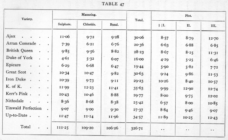
To get the other sums of squares, we'll need various aggregate values, which Fisher gives us in a separate table:

But let's derive these from the original data.
We can get the variety-wise tokens simply by asking Matlab to sum the columns:
FPV = sum(FP,2)

FPV =
   30.0600
   20.3600
   28.2300
   16.0000
   19.4400
   30.6300
   29.2300
   35.6300
   29.7700
   25.4200
   27.3700
   34.5700
Now let's check Fisher's assertion that "the value [of the sum of squared deviations] for the 12 varieties is 43.638":
x = FPV-mean(FPV)
x =
    2.8342
   -6.8658
    1.0042
  -11.2258
   -7.7858
    3.4042
    2.0042
    8.4042
    2.5442
   -1.8058
    0.1442
    7.3442
x'*x
  ans =
    392.7455
Well, 392.7455/9 = 43.6384, so Fisher's value in this case is is the variance of the data summed by variety, divided by the number of columns in the original matrix. This makes sense, because the values in the aggregated totals by variety are the sum of the nine columns, and thus are each about 9 times the original per-cell values. If we want to compare the sum of squared deviations in the two cases, we have to scale the aggregated case accordingly.
Another way to get this same number would be to subtract the "composite" sum of squares from the "treatment" sum of squares:
TT = FPV(:)'*FPV(:)/9
TT =
  1.0320e+003
TT-CC
ans =
   43.6384
What happens when we check Fisher's assertion that "according to patches, in 36 classes of 3, the value for the 36 patches is 61.078":
His table groups the columns by treatment (3 sulphate, 3 chloride, 3 basal), so we can sum patch-wise as follows:
FPP = [sum(FP(:,[1 4 7]),2) sum(FP(:,[2 5 8]),2) sum(FP(:,[3 6 9]),2)]

FPP =
    8.5700    8.7900   12.7000
    6.6300    6.8800    6.8500
    8.6700    8.2500   11.3100
    4.2900    5.2500    6.4600
    5.9000    5.8200    7.7200
    9.2400    9.8600   11.5300
   10.2600    8.4000   10.5700
    9.9900   12.9000   12.7400
    8.0000    9.7500   12.0200
    6.5700    8.0000   10.8500
    8.8400    9.4600    9.0700
   11.8900   10.2500   12.4300
And we can calculate the patch-wise sum of squared deviations this way:
x = FPP-mean(FPP(:)); x(:)'*x(:)
 ans =
  183.2355
Again, 183.2355/3 = 61.0785, so we get Fisher's answer if we scale by an appropriate factor. (Or, again again, we could subtract the "composite" sum of squares from a patch-wise sum of squares...)
So, to repeat, we've reproduced Fisher's list of sums of squared deviations:
The sum of the squares of the deviations of all the 108 values from their mean is 71.699; divided, according to patches, in 36 classes of 3, the value for the 36 patches is 61.078; dividing this again according to varieties into 12 classes of 3, the value for the 12 varieties is 43.638.
Fisher now tells us that
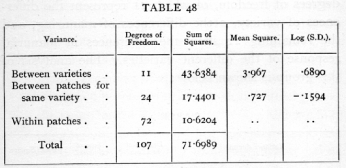
We may express the facts so far as follows:

Wait, in that "Sum of Squares" columns, 43.6384 was the sum of squared deviations for the varieties, but where did 17.4401 and 10.6204 come from? Well, the idea is that the total sum of squared deviations (71.6989) should be divided up among additive contributions from varieties, manurings, and patches-- three components, rather than just two.
Recall that the patch-wise SSD was 61.0785 -- if we subtract the variety-wise SSD of 43.6384, we get 61.0785-43.6384 = 17.4401, which is asserted to be the SSD contributed by patch variation for a given variety.
This amounts to assuming that decompositions of these scaled sums-of-squared-deviations should be additive: the SSD for variety and the SSD of patches for the same variety should add up to the SSD of patches.
Similarly, the SSD of patches and the SSD of treatments within a patch should add up to the overall sum of squared deviations for the whole dataset, which we found to be 71.6989. And indeed, 71.6989-61.0785 = 10.6204, the last number in the "Sum of Squares" column, asserted to be the SSD (of the treatments) "within patches".
Fisher has thus decomposed the overall sum of squared deviations -- the variance times the number of observations -- into a component associated with varieties, a component associated with patches, and a component associated with manurings. The next step is going to be to analyze this decomposition in order to determine the answer to one of the intitial questions about significance.
This next step starts with the column labelled "Mean Square"? The values there are exactly the second column ("Sum of Squares") divided by the first column ("Degrees of Freedom"):
3.967 = 43.6384/11
0.727 = 17.4401/24
In this context, as Wikipedia tells us, 'the number of degrees of freedom is the number of independent observations in a sample of data that are available to estimate a parameter of the population from which that sample is drawn".
In calculating the mean of 12 numbers, we have 12 independent observations, and thus 12 degrees of freedom. But in calculations based on differences from the mean value of a set of numbers, one of the degrees of freedom goes away. This is easy to see when there are two numbers: they're equidistant from the mean, by definition, and so once we've learned what one deviation is, the other one contributes no new information. In larger sets, the fact that the sum of deviations must be zero means that once we've learned n-1 deviations, the last one is redundant. (The argument for squared deviations is similar if a bit more complex.)
So the SSD for the 12 varieties has df = 11, and thus its estimated variance is the SSD/11.
In the case of the sum of squared deviations "between patches for the same variety", we've subtracted the SSD for the 12 varieties from the SSD for the 36 patches. Why does this yield 36-12 = 24 degrees of freedom, rather than 23?
One easy way to think about this is to observe that 35-11 is also equal to 24: if we lose one df from each of the SSDs, the difference in degrees of freedom is unaffected.
What about the fourth column, the one labelled "Log(S.D.)"?

That's there because Fisher didn't use the famous F distribution, named after Fisher by George Snedecor in the 1930s, but rather what he called the z distribution, which is half the natural log of the F distribution.
Thus in this case, the F test would compare 3.967/.727 → 5.4567 (the ratio of variances) to the F-distribution threshold for a significance level of .05 for a ratio of variances with 11 and 24 degrees of freedom respectively (finv(.95,11,24) → 2.2163, in Matlab-ese). Having observed that 5.4567 is larger than 2.2163, we would conclude that indeed, a celebration would be propitious, as the effect of varieties was highly "significant".
Fisher does the calculation this way:
The value of z, found as the difference of the logarithms in the last column, is nearly .85, or more than twice the 5 per cent value; the effect of variety is therefore very significant.
Here the "5 per cent value" for z would be .5*log(finv(.95,11,24)) → 0.3979
You can read on in Fisher's chapter in order to learn that the differences among patches was highly significant:
As is always found in careful field trials, local irregularities in the nature or depth of the soil materially affect the yields. In this case the soil irregularity was perhaps combined with unequal quality or quantity of the dung supplied.
And there was no significant effect of manurings:
Evidently the plants with the basal dressing had all the potash necessary, and in addition no apparent effect on the yield was produced by the difference between chloride and sulphate ions.
It's obvious why agricultural researchers -- and social and behavioral scientists -- would be impressed with this efficient use of systematically-collected evidence to decide what matters and what doesn't. And it's not surprising that a large proportion of published papers in various experimental sciences use F-tests and similar devices to determine the "significance" of effects and interactions.
But there are some dissenting voices.
You can read Harald Baayen's paper to see one class of objections, mainly concerned with the impoverished structure of the statistical models implicit in most psychologists' use of ANOVA.
And you can read various works by Deirdre McCloskey and Stephen Ziliak for a somewhat different brand of dissent, most recently in their 2008 book The cult of statistical significance. Their objections apply not just to ANOVA, but to the whole notion of "statistical significance" that R.A. Fisher pioneered. They feel that the term is misleading, since it simply evaluates the hypothesis that a certain property of a sample might have arisen by chance, without evaluating the (economic, clinical, perceptual, etc.) effects. (Thus in Fisher's potato experiment, he concluded that the effect of variety was "highly significant" without drawing any conclusions about what the expected difference in yield actually was for the various varieties.)
Here's the abstract of McCloskey & Ziliak's 2004 paper "Size matters: the standard error of regressions in the American Economic Review", Journal of Socio-Economics, 33(5), 2004
Significance testing as used has no theoretical justification. Our article in the Journal of Economic Literature (1996) showed that of the 182 full-length papers published in the 1980s in the American Economic Review 70% did not distinguish economic from statistical significance. Since 1996 many colleagues have told us that practice has improved. We interpret their response as an empirical claim, a judgment about a fact. Our colleagues, unhappily, are mistaken: significance testing is getting worse. We find here that in the next decade, the 1990s, of the 137 papers using a test of statistical significance in the AER fully 82% mistook a merely statistically significant finding for an economically significant finding. A super majority (81%) believed that looking at the sign of a coefficient sufficed for science, ignoring size. The mistake is causing economic damage: losses of jobs and justice, and indeed of human lives (especially in, to mention another field enchanted with statistical significance as against substantive significance, medical science). The confusion between fit and importance is causing false hypotheses to be accepted and true hypotheses to be rejected. We propose a publication standard for the future: “Tell me the oomph of your coefficient; and do not confuse it with merely statistical significance.”
By "significance testing" they mean determining whether a reproducible difference exists, without any concern for whether the magnitude of the difference is large enough to matter. By "oomph", they mean something like "how much the effect matters to the issue under discussion".
More on all this later...